Mathematica绘制函数图像—隐函数图像
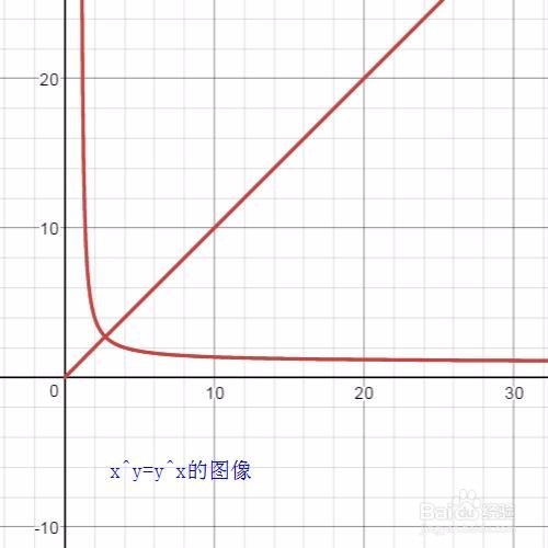
1、 有人可能要说,画不出隐函数的图像,你可以把隐函数方程化成显函数来画呀!或者转化成参数方程的形式呀!就像椭圆的参数方程是:x=sint,y=cost,这不就把椭圆的方程的“隐函数”转化为“参数方程”了吗?
对此,我只好难为他们一下了:
请尝试着把x^y=y^x转化为“非隐函数”的形式。

2、 隐函数的图像,要用ContourPlot命令函数来实现。
例如:绘制x^x+y^y=5/3的图像。
Mathematica代码是:
ContourPlot[x^x + y^y == 5/3, {x, 0, 1}, {y, 0, 1}, ImageSize -> {500, 500}]
注意格式:这里图形大小设定为500×500像素;方程x^x + y^y == 5/3之间的等号必须是双等号;x和y的绘图范围都要写出来。
运行以后得到的图形是下面第一个图。第二个图是用Desmos画出来的。


3、 其实,ContourPlot还可以绘制等高线图。
ContourPlot[x^x + y^y, {x, -0.5, 2}, {y, -0.5, 2}]
ContourPlot[x^x + y^y, {x, -0.1, 0.7}, {y, -0.1, 0.7}]
发现,当x^x + y^y的值过大的时候,图形不是封闭曲线。于是产生一个问题:要保证x^x + y^y=a的图像是封闭曲线,a的最大值和最小值分别是多少?


4、 绘制x^x + y^y + z^z ==2.3的三维图形,要用到的命令函数是ContourPlot3D。具体的格式与ContourPlot类似,唯一的区别是,多了个变量z。
代码是:
ContourPlot3D[ x^x + y^y + z^z == 2.3, {x, 0, 1.1}, {y, 0, 1.1}, {z, 0, 1.1}]
结果是一个封闭的三维曲面。
一个类似的问题:要保证x^x + y^y+z^z=a的图像是封闭曲面,a的最大值和最小值分别是多少?

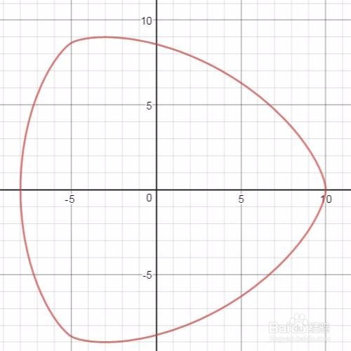
1、 有一条著名的等宽曲线,它不同于Reuleaux三角形之流。因为它不是靠许多圆弧拼成的,而是处处光滑,可以由一个隐函数方程(一个8元2次多项式)给出来。以前,我用Desmos画出来了,当时只截了个图,没有贴代码。由于方程式很长,所以,这里把代码贴出来。
Mathematica代码:
ContourPlot[(x^2 + y^2)^4 - 45 (x^2 + y^2)^3 - 41283 (x^2 + y^2)^2 + 7950960 (x^2 + y^2) + 16 (x^2 - 3 y^2)^3 + 48 (x^2 + y^2) (x^2 - 3 y^2)^2 - 720^3 + (x^2 - 3 y^2) x (16 (x^2 + y^2) ^2 - 5544 (x^2 + y^2) + 266382) == 0, {x, -10, 10}, {y, -10, 10}]
Desmos代码是:
0=\left(x^2+y^2\right)^4-45\left(x^2+y^2\right)^3-41283\left(x^2+y^2\right)^2+7950960\left(x^2+y^2\right)+16\left(x^2-3y^2\right)^3+48\left(x^2+y^2\right)\left(x^2-3y^2\right)^2+x\left(x^2-3y^2\right)\left(16\left(x^2+y^2\right)^2-5544\left(x^2+y^2\right)+266382\right)-720^3
对比结果如下:

2、 等高线图:
ContourPlot[(x^2 + y^2)^4 - 45 (x^2 + y^2)^3 - 41283 (x^2 + y^2)^2 + 7950960 (x^2 + y^2) + 16 (x^2 - 3 y^2)^3 + 48 (x^2 + y^2) (x^2 - 3 y^2)^2 - 720^3 + (x^2 - 3 y^2) x (16 (x^2 + y^2) ^2 - 5544 (x^2 + y^2) + 266382), {x, -10, 10}, {y, -10, 10}]
可以发现,当代码里的式子变大,就不是等宽曲线了(变小时,不能肯定)。于是有一个问题,怎么证明上面步骤里的曲线是等宽曲线?我不会,留着慢慢解答。

3、 关于等宽曲线的其它内容,参考《等宽曲线的理解和构造》。


1、 去掉坐标轴,用Axes->False;
去掉边框,用Frame->False;
ContourStyle 决定等高线的外形特征。
例如:
ContourPlot[x^x + y^y == 5/3, {x, 0, 1}, {y, 0, 1},
ContourStyle -> {Blue, Thickness[0.01]}, Axes -> False,
Frame -> False, ImageSize -> {500, 500}]
这是一条蓝色的曲线,宽度为0.01。

2、 PlotLabel 给图形添加标签,一般位于顶部;
LabelStyle 决定标签的外观特征。
把上面的代码加以修改:
ContourPlot[x^x + y^y == 5/3, {x, 0, 1}, {y, 0, 1},
ContourStyle -> {Blue, Thickness[0.01]}, Axes -> False,
Frame -> False, PlotLabel -> Style[x^x + y^y == 5/3, 20],
LabelStyle -> Directive[Bold, Blue], ImageSize -> {500, 500}]
于是,图形上边有了一个标签。

3、 Ticks 给出坐标轴的具体刻度值。用“非圆弧等宽曲线”为例,分“有坐标轴”和“没有坐标轴”两类。
“有坐标轴”的代码:
F[x_, y_] := (x^2 + y^2)^4 - 45 (x^2 + y^2)^3 - 41283 (x^2 + y^2)^2 + 7950960 (x^2 + y^2) + 16 (x^2 - 3 y^2)^3 + 48 (x^2 + y^2) (x^2 - 3 y^2)^2 - 720^3 + (x^2 - 3 y^2) x (16 (x^2 + y^2)^2 - 5544 (x^2 + y^2) + 266382);
ContourPlot[F[x, y] == 0, {x, -10, 10}, {y, -10, 10}, ContourStyle -> {Blue, Thickness[0.01]}, Axes -> True, Frame -> False, Ticks -> {{-10, 6, 8}, {0, 1, 6}}, PlotLabel -> F[x, y] == 0, AspectRatio -> Automatic]
“没有坐标轴”的代码:
ContourPlot[F[x, y] == 0, {x, -10, 10}, {y, -10, 10}, ContourStyle -> {Blue, Thickness[0.01]}, Axes -> False, Frame -> False, PlotLabel -> F[x, y] == 0, AspectRatio -> Automatic]
这里出现一个问题:用Mathematica给图形添加标签,如果标签特别长,如下图那样不能完整显示,应该怎么办?


4、 用虚线作为等高线,ContourStyle->Dashed;
等高线完全透明,ContourStyle->None。
代码两个:
ContourPlot[F[x, y], {x, -10, 10}, {y, -10, 10}, ContourStyle -> Dashed]
和
ContourPlot[F[x, y], {x, -10, 10}, {y, -10, 10}, ContourStyle -> None]


5、 Contours 确定等高线的密集程度。
ContourPlot[F[x, y], {x, -10, 10}, {y, -10, 10}, ContourStyle -> Dashed, Contours -> 20]
和
ContourPlot[F[x, y], {x, -10, 10}, {y, -10, 10}, ContourStyle -> None, Contours -> 20]


6、 绘制3D曲面的时候,不想要网格线,可以Mesh->None;
如果有网格线,那么MeshStyle确定网格线的模样。
代码是
ContourPlot3D[ x^x + y^y + z^z == 2.3, {x, 0, 1.1}, {y, 0, 1.1}, {z, 0, 1.1}, Axes -> False, Mesh -> None, PlotLabel -> Style[怎么能把外框去掉, Red, 30], ColorFunction -> Function[{x, y, z}, Hue[x + y + z]]]
和
ContourPlot3D[ x^x + y^y + z^z == 2.3, {x, 0, 1.1}, {y, 0, 1.1}, {z, 0, 1.1}, Axes -> False, PlotLabel -> Style[怎么能把外框去掉, Red, 30], MeshStyle -> Dashed, Mesh -> 5, ColorFunction -> Function[{x, y, z}, Hue[x + y + z]]

