图像算法:分水岭分割程序实现
1、分水岭算法思想:
分水岭算法是模拟自底向上逐渐淹没地形过程的形象理解;
①此地形中最低区域(种子区域)即盆地,
当水从盆地不断的浸入其中,则该地形由谷底向上逐渐的被淹没;
②当两个集水盆地的水将要汇合时,可在汇合处建立堤坝,直到整个地形都被淹泪侨没,从而就得到了各个堤坝(分水岭)和一个个被堤坝分开的盆地(目标物体)。
【注】:
分水岭算法的优点:
在于它可以得到单一像素宽度的连续边界,能检测出图像中粘连物体的微弱边缘;

2、OpenCV实现:
OpenCV实涛侨现了一个基于标记图层的分水岭算法;
所谓标记图层,即不用手动选择种子点,直接输入一个包含种子点的图像即可;
格式:
void watershed(InputArray image, InputOutputArray markers)
参数:
image-输入图像
markers-输入的标记图层,标记点是洪水漫冲的入口;
【注】:
要获得较好的分水岭分割效果,一般先获得最佳的种子区域;
那么如何获得标记图层呢?
3、OpenCV分水岭分割程序:
①将输入灰度图转换二值图
②findContours()函数找出图像轮廓
③将轮廓查找结果放入到markers图层中,便于访问;
④调用分水岭分割算法,显示分割结果;
#include <opencv2\opencv.hpp>
#include <opencv2\highgui\highgui.hpp>
#include <opencv2\features2d\features2d.hpp>
#include <opencv2\core\core.hpp>
using namespace std;
using namespace cv;
int main()
{
Mat srcImg = imread("raw.jpg",1);
Mat grayImg;
cvtColor(srcImg,grayImg,CV_BGR2GRAY);
Mat binaryImg = Mat::zeros(grayImg.rows,grayImg.cols,CV_8UC1);
adaptiveThreshold(grayImg,binaryImg,255,ADAPTIVE_THRESH_GAUSSIAN_C,THRESH_BINARY_INV,5,10);
namedWindow("threshold", CV_WINDOW_NORMAL);
imshow("threshold",binaryImg);
vector< vector<Point> > vContours;
vector< Vec4i > vHierarchy;
findContours(binaryImg,vContours,vHierarchy,CV_RETR_LIST,CV_CHAIN_APPROX_NONE);
Mat markersImg = Mat::zeros(grayImg.rows,grayImg.cols,CV_8UC1);
for (int idx=0;idx>=0;idx=vHierarchy[idx][0])
{
Scalar color(rand()&255,rand()&255,rand()&255);
drawContours(markersImg,vContours,idx,color,CV_FILLED,8,vHierarchy);
}
namedWindow("contours", CV_WINDOW_NORMAL);
imshow("contours",markersImg);
Mat markers;
markersImg.convertTo(markers, CV_32S);
watershed(srcImg, markers);
腊蚊屈 Mat segmentImg;
markers.convertTo(segmentImg,CV_8U);
namedWindow("segmentation_result", CV_WINDOW_NORMAL);
imshow("segmentation_result", segmentImg);
waitKey(0);
return 0;
}


4、Matlab分水岭程序实现:
clc;clear all;close all
%1.读入彩色图像 并转换成灰度图 显示%
rgb=imread('pears.png');
if ndims(rgb)==3
I=rgb2gray(rgb);
else
I=rgb;
end
figure('units','normalized','position',[0 0 1 1]);
subplot(1,2,1);imshow(rgb);title('原图');
subplot(1,2,2);imshow(I);title('灰度图');

5、接上:
%2.进行分割图像%
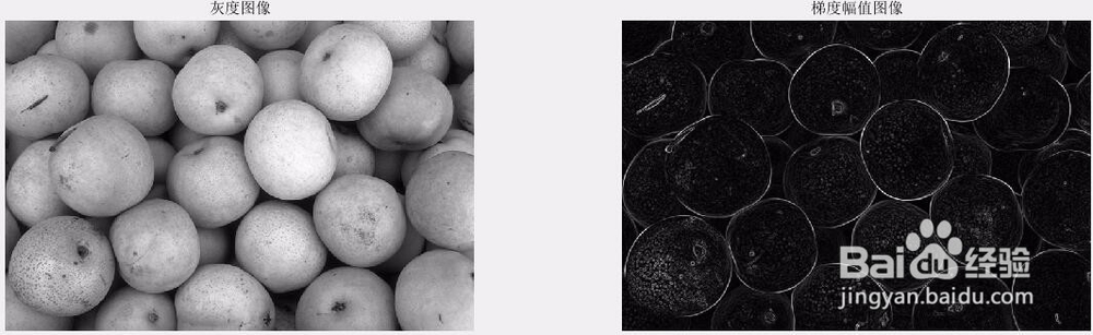
%采用sobel边缘算子对图像进行水平和垂直滤波
%求取其模值
%soble算子滤波后的图像在边界处会显示比较大的值,没有边界处的值会很小
hy = fspecial('sobel');
hx = hy';
Iy = imfilter(double(I),hy,'replicate');
Ix = imfilter(double(I),hx,'replicate');
gradmag = sqrt(Ix.^2+Iy.^2);
figure('units','normalized','position',[0 0 1 1]);
subplot(1,2,1);imshow(I,[]);title('灰度图像');
subplot(1,2,2);imshow(gradmag,[]);title('梯度幅值图像');
%可否直接对梯度幅值图像使用分水岭算法?
%直接使用分水岭算法对梯度幅值图像分割 结果往往存在过度分割的现象;
%因此 需要对前景和背景进行标记,以获得更好地分割效果
L=watershed(gradmag);
Lrgb=label2rgb(L);
figure('units','normalized','position',[0 0 1 1]);
subplot(1,2,1);imshow(gradmag,[]);title('梯度幅值图像');
subplot(1,2,2);imshow(Lrgb,[]);title('梯度幅值做分水岭变换');

6、接上:
%3.标记前景目标对象
%标记必须是前景对象内部的连接斑点像素
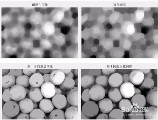
%开运算可以把结构元素小的突刺滤掉 切断细长搭接而起到分离作用
%闭运算可以把结构元素小的缺口或孔填充上 搭接段的间隔而起到连接作用
se = strel('disk',20);
Io = imopen(I,se);
figure('units','normalized','position',[0 0 1 1]);
subplot(1,2,1);imshow(I,[]);title('灰度图像');
subplot(1,2,2);imshow(Io,[]);title('开操作');
Ie = imerode(I,se);
Iobr = imreconstruct(Ie,I);
figure('units','normalized','position',[0 0 1 1]);
subplot(1,2,1);imshow(I,[]);title('灰度图像');
subplot(1,2,2);imshow(Iobr,[]);title('基于开的重建图像');
%闭操作移除较暗的斑点和枝干标记
Ioc = imclose(Io,se);
Ic = imclose(I,se);
figure('units','normalized','position',[0 0 1 1]);
subplot(2,2,1);imshow(I,[]);title('灰度图像');
subplot(2,2,2);imshow(Io,[]);title('开操作图像');
subplot(2,2,3);imshow(Ic,[]);title('闭操作图像');
subplot(2,2,4);imshow(Ioc,[]);title('开闭运算');
%采用imdilate imreconstruct 对输入图像求补 对imreconstruct输出图像求补
Iobrd = imdilate(Iobr,se);
Iobrcbr = imreconstruct(imcomplement(Iobrd),imcomplement(Iobr));
Iobrcbr = imcomplement(Iobrcbr);
figure('units','normalized','position',[0 0 1 1]);
subplot(2,2,1);imshow(I,[]);title('灰度图像');
subplot(2,2,2);imshow(Ioc,[]);title('开闭操作');
subplot(2,2,3);imshow(Iobr,[]);title('基于开的重建图像');
subplot(2,2,4);imshow(Iobrcbr,[]);title('基于闭的重建图像');
%比较Ioc和Iobrcbr,在移除小污点同时不影响对象全局形状的应用下
%基于重建的开闭操作要比标准的开闭重建更加有效
%故计算Iobrcbr的局部极大值来得到更好地前景标记
fgm = imregionalmax(Iobrcbr);
figure('units','normalized','position',[0 0 1 1]);
subplot(1,3,1);imshow(I,[]);title('灰度图像');
subplot(1,3,2);imshow(Iobrcbr,[]);title('基于重建的开闭操作');
subplot(1,3,3);imshow(fgm,[]);title('局部极大图像');
%为了帮助理解结果 叠加前景标记到原图中
It1 = rgb(:,:,1);
It2 = rgb(:,:,2);
It3 = rgb(:,:,3);
It1(fgm)=255;
It2(fgm)=0;
It3(fgm)=0;
I2 = cat(3,It1,It2,It3);
figure('units','normalized','position',[0 0 1 1]);
subplot(2,2,1);imshow(rgb,[]);title('原图像');
subplot(2,2,2);imshow(Iobrcbr,[]);title('基于重建的开闭操作');
subplot(2,2,3);imshow(fgm,[]);title('局部极大图像');
subplot(2,2,4);imshow(I2);title('局部极大叠加到原图像');
%注意 大多闭塞出和阴影对象没有被标记
se2 = strel(ones(5,5));
fgm2 = imclose(fgm,se2);
fgm3 = imerode(fgm2,se2);
figure('units','normalized','position',[0 0 1 1]);
subplot(2,2,1);imshow(Iobrcbr,[]);title('基于重建的开闭操作');
subplot(2,2,2);imshow(fgm,[]);title('局部极大图像');
subplot(2,2,3);imshow(fgm2,[]);title('基于局部极大图像的闭操作');
subplot(2,2,4);imshow(fgm3,[]);title('基于闭操作的腐蚀操作');
%这个过程会留下一些偏离的孤立像素,应该移除它们
fgm4 = bwareaopen(fgm3,20);
It1 = rgb(:,:,1);
It2 = rgb(:,:,2);
It3 = rgb(:,:,3);
It1(fgm4)=255;
It2(fgm4)=0;
It3(fgm4)=0;
I3 = cat(3,It1,It2,It3);
figure('units','normalized','position',[0 0 1 1]);
subplot(2,2,1);imshow(I2,[]);title('局部极大值叠加到原图像');
subplot(2,2,2);imshow(fgm3,[]);title('闭腐蚀操作');
subplot(2,2,3);imshow(fgm4,[]);title('去除小斑点操作');
subplot(2,2,4);imshow(I3,[]);title('修改局部极大值叠加到原图像');


7、接上:
%4.计算背景标记
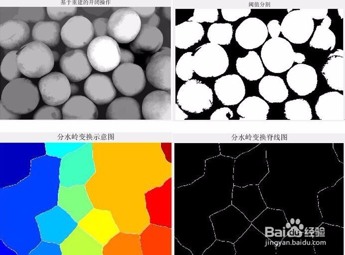
%在Iobrcbr中 暗像素属于北京 阈值操作
bw = im2bw(Iobrcbr,graythresh(Iobrcbr));
figure('units','normalized','position',[0 0 1 1]);
subplot(1,2,1);imshow(Iobrcbr,[]);title('基于重建的开闭操作');
subplot(1,2,2);imshow(bw,[]);title('阈值分割');
%背景像素在黑色区域 理想情形下 不必要求背景标记太接近于要分割的对象边缘;
%通过计算‘骨架影响范围’来细化背景,或者SKIZ,bw的前景;
%采用bw的距离变换得分水岭变换实现;
%然后寻找结果的分水岭脊线DL==0
%D=bwdist(BW)计算欧几里得距离公式
%BW可以由任意维数,
%D与BW有同样的大小
D=bwdist(bw);
DL=watershed(D);
bgm = DL == 0;
figure('units','normalized','position',[0 0 1 1]);
subplot(2,2,1);imshow(Iobrcbr,[]);title('基于重建的开闭操作');
subplot(2,2,2);imshow(bw,[]);title('阈值分割');
subplot(2,2,3);imshow(label2rgb(DL),[]);title('分水岭变换示意图');
subplot(2,2,4);imshow(bgm,[]);title('分水岭变换脊线图');
8、接上:
%5.计算分水岭分割
%imimposemin用来修改图像 使特定要求位置局部最小
%imimposemin用来修改梯度幅值图像 在前景和背景标记像素局部极小
gradmag2 = imimposemin(gradmag,bgm|fgm4);
figure('units','normalized','position',[0 0 1 1]);
subplot(2,2,1);imshow(bgm,[]);title('分水岭变换脊线图');
subplot(2,2,2);imshow(fgm4,[]);title('前景标记');
subplot(2,2,3);imshow(gradmag,[]);title('梯度幅值图像');
subplot(2,2,4);imshow(gradmag2,[]);title('梯度幅值修改图像');

9、接上:
%6.基于分水岭图像的分割计算
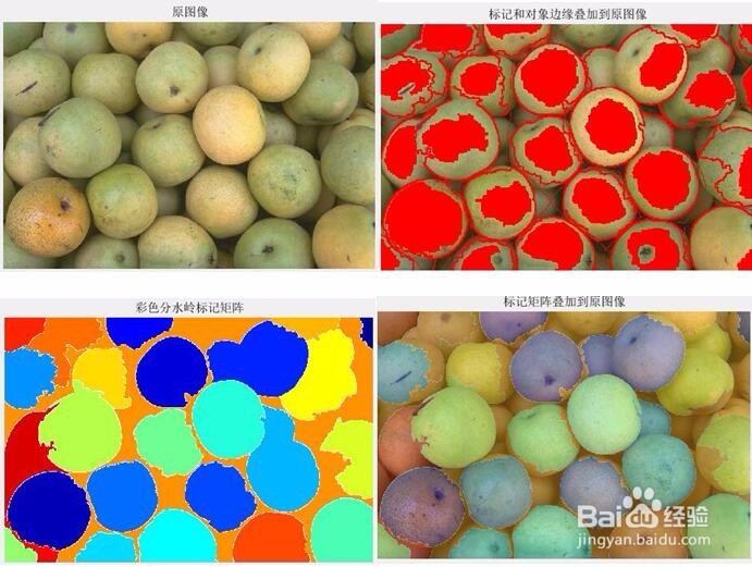
%查看结果 叠加前景标记、背景标记 分割对象边界
%采用膨胀实现某些要求 比如对象边界更加清晰可见
%对象边界定位于L==0的位置;
L=watershed(gradmag2);
It1 = rgb(:,:,1);
It2 = rgb(:,:,2);
It3 = rgb(:,:,3);
fgm5 = imdilate(L==0,ones(3,3)) | bgm | fgm4;
It1(fgm5)=255;
It2(fgm5)=0;
It3(fgm5)=0;
I4=cat(3,It1,It2,It3);
figure('units','normalized','position',[0 0 1 1]);
subplot(1,2,1);imshow(rgb,[]);title('原图像');
subplot(1,2,2);imshow(I4,[]);title('标记和对象边缘叠加到原图像');
%可视化说明了前景和后景标记如何影响结果
%在几个位置 部分的较暗对象与它们邻近较亮对象相融合,
%这是因为受遮挡的对象没有前景标记
%另一可视化技术 将标记矩阵作为彩色图象显示
%
Lrgb = label2rgb(L,'jet','w','shuffle');
figure('units','normalized','position',[0 0 1 1]);
subplot(1,2,1);imshow(rgb,[]);title('原图像');
subplot(1,2,2);imshow(Lrgb);title('彩色分水岭标记矩阵');
%使用透明度来叠加这个伪彩色标记矩阵在原亮度图像上进行显示
figure('units','normalized','position',[0 0 1 1]);
subplot(1,2,1);imshow(rgb,[]);title('原图像');
subplot(1,2,2);imshow(rgb,[]);hold on;
himage = imshow(Lrgb);
set(himage,'AlphaData',0.3);
title('标记矩阵叠加到原图像');
10、完整程序如下:
clc;clear all;close all
%1.读入彩色图像 并转换成灰度图 显示%
rgb=imread('pears.png');
I=rgb2gray(rgb);
%2.进行分割图像%
hy = fspecial('sobel');
hx = hy';
Iy = imfilter(double(I),hy,'replicate');
Ix = imfilter(double(I),hx,'replicate');
gradmag = sqrt(Ix.^2+Iy.^2);
figure('units','normalized','position',[0 0 1 1]);
subplot(1,2,1);imshow(I,[]);title('灰度图像');
subplot(1,2,2);imshow(gradmag,[]);title('梯度幅值图像');
%3.标记前景目标对象
%有多种方法可以获得前景标记 但标记必须是前景对象内部的连接斑点像素
%开运算可以把结构元素小的突刺滤掉 切断细长搭接而起到分离作用
%闭运算可以把结构元素小的缺口或孔填充上 搭接段的间隔而起到连接作用
se = strel('disk',20);
Io = imopen(I,se);
Ie = imerode(I,se);
Iobr = imreconstruct(Ie,I);
Ioc = imclose(Io,se);
Ic = imclose(I,se);
%采用imdilate imreconstruct 对输入图像求补 对imreconstruct输出图像求补
Iobrd = imdilate(Iobr,se);
Iobrcbr = imreconstruct(imcomplement(Iobrd),imcomplement(Iobr));
Iobrcbr = imcomplement(Iobrcbr);
%比较Ioc和Iobrcbr,在移除小污点同时不影响对象全局形状的应用下
%基于重建的开闭操作要比标准的开闭重建更加有效
%计算Iobrcbr的局部极大值来得到更好地前景标记
fgm = imregionalmax(Iobrcbr);
%为了帮助理解结果 叠加前景标记到原图中
It1 = rgb(:,:,1);It2 = rgb(:,:,2);It3 = rgb(:,:,3);
It1(fgm)=255;It2(fgm)=0;It3(fgm)=0;
I2 = cat(3,It1,It2,It3);
%注意 大多闭塞出和阴影对象没有被标记 即在结果中将不会得到合理的分割
%清理标记斑点的边缘 然后收缩它们
%闭操作和腐蚀操作完成
se2 = strel(ones(5,5));
fgm2 = imclose(fgm,se2);
fgm3 = imerode(fgm2,se2);
%这个过程会留下一些偏离的孤立像素,应该移除它们
%采用bwareaopen移除少于特定像素个数的斑点
fgm4 = bwareaopen(fgm3,20);
It1 = rgb(:,:,1);
It2 = rgb(:,:,2);
It3 = rgb(:,:,3);
It1(fgm4)=255;
It2(fgm4)=0;
It3(fgm4)=0;
I3 = cat(3,It1,It2,It3);
%4.计算背景标记
%在Iobrcbr中 暗像素属于北京 阈值操作
bw = im2bw(Iobrcbr,graythresh(Iobrcbr));
figure('units','normalized','position',[0 0 1 1]);
subplot(1,2,1);imshow(Iobrcbr,[]);title('基于重建的开闭操作');
subplot(1,2,2);imshow(bw,[]);title('阈值分割');
%背景像素在黑色区域 理想情形下 不必要求背景标记太接近于要分割的对象边缘;
%然后寻找结果的分水岭脊线DL==0
D=bwdist(bw);
DL=watershed(D);
bgm = DL == 0;
%5.计算分水岭分割
%imimposemin用来修改图像 使特定要求位置局部最小
gradmag2 = imimposemin(gradmag,bgm|fgm4);
%6.基于分水岭图像的分割计算
%对象边界定位于L==0的位置;
L=watershed(gradmag2);
It1 = rgb(:,:,1);
It2 = rgb(:,:,2);
It3 = rgb(:,:,3);
fgm5 = imdilate(L==0,ones(3,3)) | bgm | fgm4;
It1(fgm5)=255;
It2(fgm5)=0;
It3(fgm5)=0;
I4=cat(3,It1,It2,It3);
%另一可视化技术 将标记矩阵作为彩色图象显示
Lrgb = label2rgb(L,'jet','w','shuffle');
%使用透明度来叠加这个伪彩色标记矩阵在原亮度图像上进行显示
figure('units','normalized','position',[0 0 1 1]);
subplot(1,2,1);imshow(rgb,[]);title('原图像');
subplot(1,2,2);imshow(rgb,[]);hold on;
himage = imshow(Lrgb);
set(himage,'AlphaData',0.3);
title('标记矩阵叠加到原图像');