用Mathematica绘制流量图（StreamPlot）

1、绘制{y,-x}场里面的流线。

StreamPlot[{y, -x}, {x, -3, 3}, {y, -3, 3}]

这个图看起来就像是一组同心圆。

2、增加流线的长度和箭头的大小。

StreamPlot[{y, -x}, {x, -3, 3}, {y, -3, 3}, StreamScale -> 0.16]

3、每一圈用一个箭头：

StreamPlot[{y, -x}, {x, -3, 3}, {y, -3, 3}, StreamScale -> Full]

4、绘制流量密度图：

StreamDensityPlot[{y, -x}, {x, -3, 3}, {y, -3, 3}, 

 StreamStyle -> White, FrameStyle -> Blue, Background -> Pink, 

 ColorFunction -> Hue]

5、用Cos[x y]作为着色方案：

StreamDensityPlot[{{y, -x}, Cos[x y]}, {x, -3, 3}, {y, -3, 3}, 

 MaxRecursion -> 2, ColorFunction -> Hue, StreamStyle -> White]

6、StreamPlot的本质，可以通过下面的方法，进行查看：

a = StreamPlot[{{x, y}, {y, -x}}, {x, -3, 3}, {y, -3, 3}]

a[[1]]

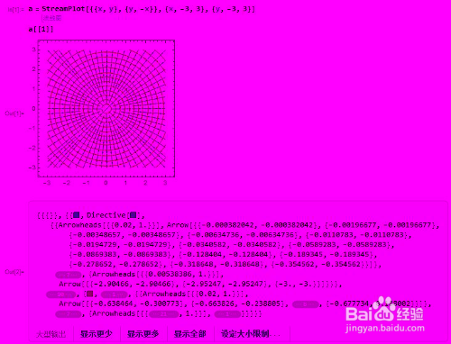
7、用Graphics画出这个流量图：

Graphics[a[[1]]